How to Make Stock Price Predictions Using Reinforcement Learning?

Analyzing the stock market using artificial intelligence has been a work in progress recently. Here, we’ll discuss how you can develop an AI stock prediction model using reinforcement learning. 

Analyzing the behavior of the stock market has been a subject of interest and challenge in the AI industry. Data scientists, market analysts, and financial experts have been curious to determine whether it is possible to overcome these challenges. The biggest concern is the need for an extra large dataset to build a predictive system based on supervised learning algorithms. 

Furthermore, even the most advanced technologies seem to be inadequate to accurately predict the changing prices in the stock market. Yet, accurate AI stock price prediction could be possible without relying on large datasets. 

In this blog, we’ll try to identify the challenges of stock market prediction and understand if we can use reinforcement learning for stock prediction and data analysis in Python, that too, using limited or no data to train the algorithm. 

Before we proceed to read more about stock price prediction using machine learning, let’s understand more about the data analysis methods used to process stock market data. 

Types of Data Analysis Techniques Used on Share Market Data 

The stock market data is analyzed in different techniques. These are categorized as – Time Series Analysis and Statistical Data Analysis.

1. Time Series Analysis 

A time series is defined as a sequence of data points that appear/ occur in successive order in a given period. It is the opposite of cross-sectional data, where the events that occur at a specific time point are captured. 

The time series analysis tracks the movement of the chosen data points over the specified period. The data points are usually the price of the stock/ share/ security. The prices are collected at regular intervals to analyze the patterns. 

There are various techniques to perform the time series analysis on stock market data. Let’s check them out in brief. 

a. Moving Averages: 

The moving average of a stock is calculated to smooth the price data and constantly update the average price. In finance, the MA (moving average) is considered a stock indicator and is used in technical analysis. The short-term price fluctuations are mitigated in this process. The MA is further divided into the following: 

i. Simple Moving Average (SMA) 

SMA is calculated using the arithmetic mean for a given set of values over a specific period. Here, the set of values is the stock prices. These are then added and divided by the number of prices in the set. 

Formula: A1+ A2+ A3+… Ann

Here, A= average in the period; nn= number of periods; SMA= n  

ii. Exponential Moving Average (EMA) 

The EMA gives more importance to recent prices to make the average price more relevant based on the new information. The SMA is calculated first to use in the EMA formula. 

The smoothing factor is calculated next to determine the weighting of EMA- 2/(selected period+1).

Formula: EMAt= [Vt×(1+ds)]+EMAy×[1−(1+ds)]

Here, EMAt= today’s EMA; Vt= today’s value; EMAy= yesterday’s EMA; ds= smoothing (number of days)

Some other types of moving averages are: 

• Double Exponential Moving Averages (DEMA)
• Weighted Moving Averages (WMA)
• Time Moving Average (TMA) 

b. ARIMA: 

It is another approach to time series forecasting. ARIMA and exponential smoothing are widely used methods as they offer a complementary approach to the problem. ARIMA describes the auto-correlations in data, while exponential smoothing relies on seasonality in data and trend description. 

c. Box Jenkins Model: 

This model can analyze different types of time series data for forecasting. It is a mathematical model that uses inputs from specified time series to forecast data ranges. The Box Jenkins model determines the outcomes based on the differences between data points. It identifies trends for forecasting stock prices using autoregression, moving averages, and seasonal differences. 

d. Rescaled Range Analysis: 

It is a statistical technique developed to assess the magnitude and nature of data variability over a certain period. The rescaled range analysis method is used to identify and evaluate persistence, randomness, and mean reversion based on the time series data from the stock markets. This insight is used to make proper investment strategies. 

2. Statistical Data Analysis 

• Mode: 

It is the common value that occurs in the dataset. 

• Median: 

It is the middle number in the dataset. For example, in 4, 6, 7, 9, and 11, the median is 7. 

• Arithmetic Mean:

It is the average value of the dataset. 

• Normal Distribution: 

It is also called standard normal distribution or Gaussian distribution model. It is charted along the horizontal axis, representing the total value spectrum in the dataset. The values of half the dataset will be higher than the mean, while the other half will be longer than the mean. And the other data points will be around the mean, with a few lying on extreme/ tail ends on both sides. 

• Skewness:  

It measures the asymmetry/ symmetry of the price/ data point distribution. The skewness will be zero in a standard normal distribution. A negative skewness will lead to a distorted bell curve on the left, while positive skewness will cause a distorted bell curve on the right side. 

What is Reinforcement Learning?

It is an area of machine learning that takes the appropriate action to maximize returns for a given situation. Many software applications and machines use reinforcement learning (RL) to identify the best behavior/ path to arrive at the desired result for a specific situation. 

Reinforcement learning is different from supervised learning. In the latter, the training data is the answer key to training the model with the correct answer. However, in RL, the reinforcement agent decides which task to perform, as there is no specific answer used for training. It allows machine learning developers to train the algorithm without using a dataset. The algorithm will learn from experience and improve itself over time. 

What are the Different Datasets Available for Stock Market Predictions?

Fortunately, there are a few datasets available to train the algorithms. Developers can access the datasets from the following: 

NIFTY-50 Stock Market Data 

The data is available from 1st January 2000 to 31st April 2021. It provides the price history and trading volumes of the fifty stocks indexed on NIFTY 50 from the National Stock Exchange (NSE) in India. The datasets have day-level pricing and trading values for each stock. They are provided in a .cvs file with a metadata file for additional information. 

Yahoo Finance 

Yahoo Finance has a vast collection of the latest information on trends, prices, and patterns in the global stock market. 

National Stock Exchange 

NSE Data & Analytics Limited provides data and info-vending services. It is previously known as DotEx International Limited, a separate setup dedicated to providing datasets and analytics. The Capital Market Segment data & market quotes, Currency Derivative Market Segment (CDS), Futures and Options Segment (F&O), Corporate Data, Corporate Bond Market data and Securities Lending & Borrowing Market (SLBM), and Wholesale Debt Market Segment (WDM) data is provided in these datasets. 

How is Python Used for Stock Trading?     

Python is a popular programming language. It is used to develop models in different niches and has become a go-to choice for creating algorithms for stock trading. It is an open-source package and easy to use when building complex statistical models. Python allows developers to develop their own data connectors, execute mechanisms, run backtesting, and optimize testing modules. 

How to Predict the Future Price of Stock Using Python?

Step1: Importing necessary libraries

import numpy as np

import pandas as pd

import matplotlib.pyplot as plt

import seaborn as sns

sns.set()

!pip install yfinance --upgrade --no-cache-dir

from pandas_datareader import data as pdr

import fix_yahoo_finance as yf

from collections import deque

import random

import tensorflow.compat.v1 as tf

tf.compat.v1.disable_eager_execution()

Step 2: Reading Stock Data

In this analysis, we used yahoo finance open-source data,

yf.pdr_override()

# df_full = pdr.get_data_yahoo("FB", start="2018-01-01", end="2019-01-01").reset_index()

# df_full.to_csv('FB.csv',index=False)

df_full= pd.read_csv('/content/INFY.NS.csv')

df_full.head()

Step 3: Creating Reward and loss for Stock market rules:

df= df_full.copy()

name = 'Q-learning agent'

class Agent:

    def__init__(self, state_size, window_size, trend, skip, batch_size):

        self.state_size = state_size

        self.window_size = window_size

        self.half_window = window_size // 2

        self.trend = trend

        self.skip = skip

        self.action_size = 3

        self.batch_size = batch_size

        self.memory = deque(maxlen = 1000)

        self.inventory = []

        self.gamma = 0.95

        self.epsilon = 0.5

        self.epsilon_min = 0.01

        self.epsilon_decay = 0.999

        tf.reset_default_graph()

        self.sess = tf.InteractiveSession()

        self.X = tf.placeholder(tf.float32, [None, self.state_size])

        self.Y = tf.placeholder(tf.float32, [None, self.action_size])

        feed = tf.layers.dense(self.X, 256, activation = tf.nn.relu)

        self.logits = tf.layers.dense(feed, self.action_size)

        self.cost = tf.reduce_mean(tf.square(self.Y - self.logits))

        self.optimizer = tf.train.GradientDescentOptimizer(1e-5).minimize(

            self.cost

        )

        self.sess.run(tf.global_variables_initializer())

    defact(self, state):

        if random.random() <= self.epsilon:

            return random.randrange(self.action_size)

        return np.argmax(

            self.sess.run(self.logits, feed_dict = {self.X: state})[0]

        )

    defget_state(self, t):

        window_size = self.window_size + 1

        d = t - window_size + 1

        block = self.trend[d : t + 1] if d >= 0else -d * [self.trend[0]] + self.trend[0 : t + 1]

        res = []

        for i inrange(window_size - 1):

            res.append(block[i + 1] - block[i])

        return np.array([res])

    defreplay(self, batch_size):

        mini_batch = []

        l = len(self.memory)

        for i inrange(l - batch_size, l):

            mini_batch.append(self.memory[i])

        replay_size = len(mini_batch)

        X = np.empty((replay_size, self.state_size))

        Y = np.empty((replay_size, self.action_size))

        states = np.array([a[0][0] for a in mini_batch])

        new_states = np.array([a[3][0] for a in mini_batch])

        Q = self.sess.run(self.logits, feed_dict = {self.X: states})

        Q_new = self.sess.run(self.logits, feed_dict = {self.X: new_states})

        for i inrange(len(mini_batch)):

            state, action, reward, next_state, done = mini_batch[i]

            target = Q[i]

            target[action] = reward

            ifnot done:

                target[action] += self.gamma * np.amax(Q_new[i])

            X[i] = state

            Y[i] = target

        cost, _ = self.sess.run(

            [self.cost, self.optimizer], feed_dict = {self.X: X, self.Y: Y}

        )

        ifself.epsilon >self.epsilon_min:

            self.epsilon *= self.epsilon_decay

        return cost

    defbuy(self, initial_money):

        starting_money = initial_money

        states_sell = []

        states_buy = []

        inventory = []

        state = self.get_state(0)

        for t inrange(0, len(self.trend) - 1, self.skip):

            action = self.act(state)

            next_state = self.get_state(t + 1)

            if action == 1and initial_money >= self.trend[t] and t < (len(self.trend) - self.half_window):

                inventory.append(self.trend[t])

                initial_money -= self.trend[t]

                states_buy.append(t)

                print('day %d: buy 1 unit at price %f, total balance %f'% (t, self.trend[t], initial_money))

            elif action == 2andlen(inventory):

                bought_price = inventory.pop(0)

                initial_money += self.trend[t]

                states_sell.append(t)

                try:

                    invest = ((close[t] - bought_price) / bought_price) * 100

                except:

                    invest = 0

                print(

                    'day %d, sell 1 unit at price %f, investment %f %%, total balance %f,'

                    % (t, close[t], invest, initial_money)

                )

            state = next_state

        invest = ((initial_money - starting_money) / starting_money) * 100

        total_gains = initial_money - starting_money

        return states_buy, states_sell, total_gains, invest

    deftrain(self, iterations, checkpoint, initial_money):

        for i inrange(iterations):

            total_profit = 0

            inventory = []

            state = self.get_state(0)

            starting_money = initial_money

            for t inrange(0, len(self.trend) - 1, self.skip):

                action = self.act(state)

                next_state = self.get_state(t + 1)

                if action == 1and starting_money >= self.trend[t] and t < (len(self.trend) - self.half_window):

                    inventory.append(self.trend[t])

                    starting_money -= self.trend[t]

                elif action == 2andlen(inventory) >0:

                    bought_price = inventory.pop(0)

                    total_profit += self.trend[t] - bought_price

                    starting_money += self.trend[t]

                invest = ((starting_money - initial_money) / initial_money)

                self.memory.append((state, action, invest, 

                                    next_state, starting_money < initial_money))

                state = next_state

                batch_size = min(self.batch_size, len(self.memory))

                cost = self.replay(batch_size)

            if (i+1) % checkpoint == 0:

                print('epoch: %d, total rewards: %f.3, cost: %f, total money: %f'%(i + 1, total_profit, cost,

                                                                                  starting_money))

Step 4: Training of Reinforcement learning model on your defined rules

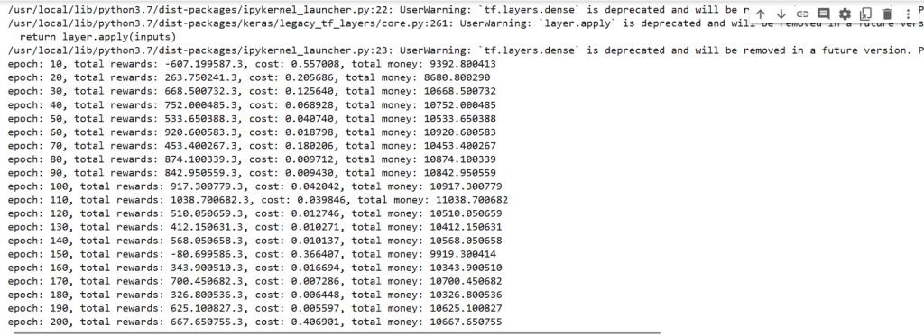
close = df.Close.values.tolist()

initial_money = 10000

window_size = 30

skip = 1

batch_size = 32

agent = Agent(state_size = window_size, 

              window_size = window_size, 

              trend = close, 

              skip = skip, 

              batch_size = batch_size)

agent.train(iterations = 200, checkpoint = 10, initial_money = initial_money)

Output:

Step 5: Checking and predicting results Reinforcement learning model on next 100 days

close = df.Close.values.tolist()

initial_money = 10000

window_size = 30

skip = 1

batch_size = 32

agent = Agent(state_size = window_size, 

              window_size = window_size, 

              trend = close, 

              skip = skip, 

              batch_size = batch_size)

agent.train(iterations = 200, checkpoint = 10, initial_money = initial_money)

Output:

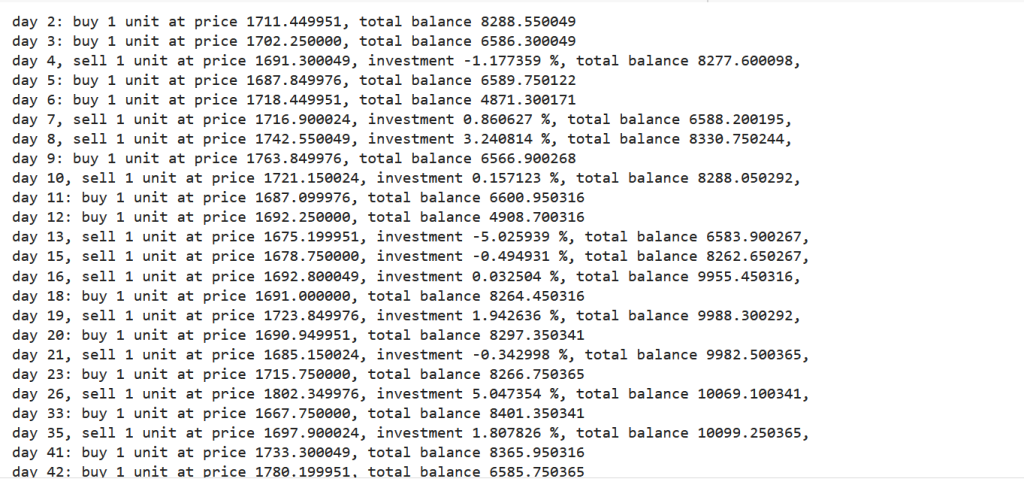
fig = plt.figure(figsize = (15,5))

plt.plot(close, color='r', lw=2.)

plt.plot(close, '^', markersize=10, color='m', label = 'buying signal', markevery = states_buy)

plt.plot(close, 'v', markersize=10, color='k', label = 'selling signal', markevery = states_sell)

plt.title('total gains %f, total investment %f%%'%(total_gains, invest))

plt.legend()

plt.savefig(name+'.png')

plt.show()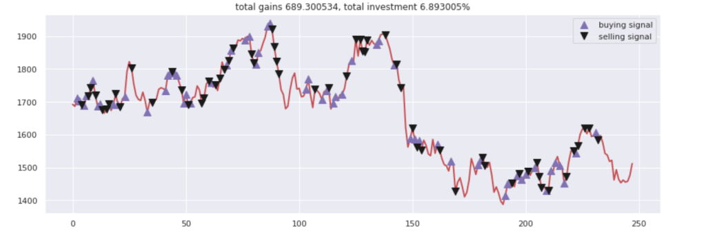

Conclusion 

You can always hire artificial intelligence solution providers to develop stock price prediction models using regressive learning. The models will learn and improve themselves as you continue to feed data and use them for predictions. 

The day is not far when AI engineers develop an accurate stock predictor to forecast the upcoming changes in prices to help investors make better decisions. This also helps with risk management and minimizing the after-effects of a market crash in case of global calamities. 

Stock Market Terminologies

Stock Market: A stock market contains several exchanges like the NASDAQ, the New York Stock Exchange, etc. Stocks are listed on the exchange and available for buyers and sellers to make a transaction. 

The exchange is a place that brings buyers and sellers together to share, trade, sell, and buy stocks. It also monitors the demand and supply of each stock and the subsequent changes in the price of the stock. A stock is a share released by a company available to the public for purchase/ selling. 

In simple terms, the stock market is a collection of exchanges that facilitate the buying and selling of shares listed by companies. The transactions happen formally as the OTC (over-the-counter) marketplaces are guided by strict regulations. The stock market is interchangeably used with the term stock exchange. Traders can buy or sell the stock on one or many exchanges. 

Broker: A person who acts as a third party between the buyer and seller. Many traders rely on stock brokers to complete the transactions on the exchanges. 

Bid: It is the amount you intend to/ are willing to pay for a stock listed on the exchange. 

Buy: It implies the act of buying shares of a company or taking a position in it. 

Sell: Handing over your stock in exchange for money. It also refers to cutting losses by getting rid of stock with decreasing prices. 

Bull: It is a stock market trend/ condition where the prices are expected to rise high. 

Bear: It is the opposite of bull and a condition of the stock market where the investors expect the prices to fall. 

Portfolio: A collection of financial investments a person owns. 

Exchange: A marketplace where different stocks and investments are traded. 

Going Long: It refers to placing a bet on the stock price that will increase. This allows you to buy for less (low) and sell for a higher price. 

Volatility: It is the frequency with which the stock prices move up or down. Stock markets have high volatility as the prices change fast.

Rohit Narain

Rohit is a Data Scientist at DataToBiz, having over 5+ years of experience in the field of Data Science, Machine Learning and NLP. He has published over 5 research papers in reputed International Journals and National conferences. When not working, you can find him engrossed in designing automobiles and learning about new innovative technologies.