Quantum computing is a fascinating concept in the science and technology industry. There’s a huge scope to use quantum computing in daily business processes in the future. We’ll discuss quantum computing concepts and see how it’s implemented using Python.
Quantum physics, as such, is a highly complex and extensive subject. The theories and concepts of quantum physics can confuse most of us, including the experts. However, researchers are making progress in utilizing the concepts of quantum physics in computing and building systems.
Quantum computation might sound like something from the future, but we are very much proceeding in that direction, albeit with tiny steps. IBM, Microsoft, and D-Wave Systems (partnering with NASA) have developed quantum computers in the cloud for public use. Yes, you can actually use a quantum computer from the cloud for free.
Of course, it’s easier said than done. Quantum computing technology is not a substitute for classic computing. It’s an extension or a diversification, where classic computing and quantum computing go hand in hand. Given how building a single quantum computer can cost thousands of dollars, using the cloud version is the best choice for us. But where does Python come into the picture? And what exactly is quantum computing?
Let’s explore this topic further and understand how to implement quantum computing concepts in Python.
The term ‘Quantum’ comes from Quantum Mechanics, which is the study of the physical properties of the nature of electrons and photons in physics. It is a framework to describe and understand the complexities of nature. Quantum computing is the process of using quantum mechanics to solve highly complicated problems.
We use classic computing to solve problems that are difficult for humans to solve. Now, we use quantum computing to solve problems that classic computing cannot solve. Quantum computing works on a huge volume of complex data in quick time.
The easiest way to describe quantum computing would be by calling it complicated computation. It is a branch of Quantum Information Science and works on the phenomena of superposition and entanglement.

The smallest particles in nature are considered quantum. Electrons, photons, and neutrons are quantum particles.
Superposition is when the quantum system is present in more than one state at the same time. It’s an inherent ability of the quantum system. We can consider the time machine as an example to explain superposition. The person in the time machine is present in more than one place at the same time. Similarly, when a particle is present in multiple states at once, it is called superposition.
Entanglement is the correlation between the quantum particles. The particles are connected in a way that even if they were present at the opposite ends of the world, they’ll still be in sync and ‘dance’ simultaneously. The distance between the particles doesn’t matter as the entanglement between them is very strong. Einstein had described this phenomenon as ‘spooky action at a distance’.

A quantum computer is a device/ system that performs quantum calculations. It stores and processes data in the form of Qubits (Quantum Bits). A quantum computer can speed up the processes of classic computing and solve problems that are beyond the scope of a classical computer.
If the classical computer takes five seconds to solve a complex mathematical problem like (689*12547836)/4587, the quantum computer will take only 0.005 seconds to give you the answer.
A quantum bit is a measure of data storage unit in quantum computers. The quantum bit is a subatomic particle that can be made of electrons or photons. Every quantum bit or Qbit adheres to the principles of superposition and entanglement. This makes things hard for scientists to generate Qbits and manage them. That’s because Qbits can show multiple combinations of zeros and ones (0 & 1) at the same time (superposition).
Scientists use laser beams or microwaves to manipulate Qbits. Though the final result collapses to the quantum state of 0 or 1, the concept of entanglement is in force. When the two bits of the pair are placed at a distance, they are still connected to each other. A change in the state of one Qbit will automatically result in the change of state for the related Qbit.
Such connected groups of Qbits are powerful compared to single binary digits used in classical computing.
Since you have a basic idea of quantum computing, it’s time to delve into the differences between classical computing and quantum computing. These differences can be categorized based on the physical structure and working processes.
In classical/ conventional computing, the electric circuits can be only in a single state at any given point in time. The circuits follow the laws of classical physics. In quantum computing, the particles follow the rules of superposition and entanglement and adhere to the laws of quantum mechanics.
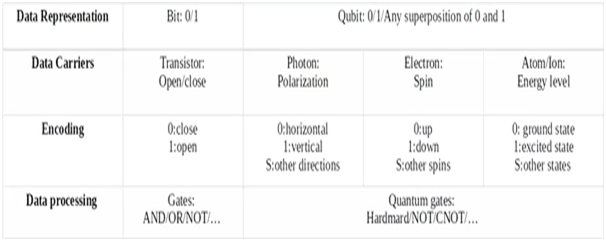
The information in classical computing is stored as bits (0 and 1), based on voltage/ charge. The binary codes represent information in conventional computing. The same is stored as Qubits or Qbit in quantum computing polarization of a photon or the spin of an electron. The Qbits include the binary code (0 & 1) and their superposition states to represent information.
Conventional computers use CMOS transistors as basic building blocks. Data is processed in the CPU (Central Processing Unit), which contains an ALU (Arithmetic and Logic Unit), Control Unit, and Processor Registers.
Quantum computers use SQUID (Superconducting Quantum Interference Device) or quantum transistors as basic building blocks. Data is processed in QPU (Quantum Processing Unit) with interconnected Qbits.
The way data is represented is the major difference between a classical computer and a quantum computer.
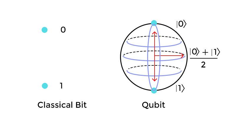
The bits in classical computing can take the value of either 0 or 1. The Qbits in quantum computing can take the value of 0 or 1 or both simultaneously in a superposition state. A Qbit is a quantum bit that can be a photon, electron, ion/ atom.
The unique ability of a Qbit to exist in the discrete states of 0 or 1 or both in superposition makes quantum computers a million times faster and more powerful than classical computers.
Quantum computing is used in the following areas:
Quantum computing can be used to solve the challenges of optimization. Brands like Airbus, JP Morgan, and Daimler work on quantum computing and test their systems for better optimization. It can be implemented in various industries for an array of purposes. Let’s take a brief look at each:
| Industry | Companies |
| Automotive | Daimler, BMW, Volkswagen, Bosch, and Ford |
| Insurance | Fenox Venture Capital and JP Morgan |
| Logistics | Amazon and Ali Baba Group |
| IT/ Software | Amazon, Microsoft, IBM, Accenture, Google, Zapata Computing, and Honeywell |
| Finance | A&E Investments, Goldman Sachs, Airbus Ventures, Bloomberg Beta, Fenox Venture Capital, Alchemist Accelerator, Felicis Ventures, Amadeus Capital Partners, DCVC (Data Collective), and Entrepreneur First (EF) |
| Energy | Quix, Hitachi, Xanadu Quantum Technologies, Qunnect Inc, Raytheon BBN, Aegiq, and Alice &Bob |
| Pharma | D-Wave Solutions, IBM, and 1QBit |
Quantum machine learning (QML) relies on two major concepts- quantum data and hybrid quantum-classical models. Let’s read more about the concepts.
Quantum data is the data that occurs in the natural or artificial quantum system or is generated by a quantum computer (data from Sycamore processor for Google’s demonstration is one example). Quantum data shows signs of superposition and entanglement. This leads to joint probability distributions, which require a huge amount of classical computing power for processing and storing.
A quantum supremacy experiment revealed that extremely complex joint probability distribution of 253 Hilbert space could be sampled using quantum computing.
NISQ processors generate noisy and entangled quantum data right before the measurement occurs. Heuristic ML models are created to extract maximum information out of the noisy data. The models are developed using the TensorFlow Quantum (TFQ) library. These models can disentangle and generalize correlations in quantum data. In turn, it leads to more opportunities that help improve the existing quantum algorithms or create new ones.
Below listed are the ways to generate quantum data using quantum devices:
It refers to extracting data and information about chemical structures and dynamics. It can be used in computational chemistry, material science, discovering drugs, and computational biology.
Hybrid quantum-classical models that are trained to perform error mitigation, calibration, and optimal open or closed-loop control, including error detection and correction strategies.
Modeling and designing superconductivity with high temperatures or other matter states show signs of many-body quantum effects.
High precision measurements used in small-scale quantum devices for quantum sensing and quantum imaging. It can be improved using variational quantum models.
Uses ML (machine learning) to discriminate non-orthogonal quantum states through the construction of quantum receivers, structured quantum repeaters, and purification units, and design application.
Though a quantum model can generalize and represent data with a quantum mechanical origin, it still cannot generalize quantum data using a quantum processor alone. This is because the near-quantum processors are noisy and limited. NISQ processors should work in tandem with quantum processors to make it an efficient model.
Luckily, TensorFlow supports heterogeneous computing across CPUs, GPUs, and TPUs. It is also used as the base to experiment on hybrid quantum-classical algorithms.
A Quantum Neural Network (QNN) describes a parameterized quantum computing model usually executed on a quantum computer. QNN is interchangeably used with parameterized quantum circuits (PQC).
QNN is a machine learning algorithm that combines artificial neural networks and quantum computing. The term has been vastly used to describe a range of ideas and concepts, be it a quantum computer emulating the concepts of neural nets or describing a quantum circuit that can be trained but with little resemblance to the multi-layer perceptron structure.
In the 1990s, quantum physicists tried to create quantum versions of feed-forward and recurrent neural networks. The aim was to try and translate modular structure and the nonlinear activation functions of neural networks into quantum algorithm language. That said, the chain of linear and nonlinear computations were not natural in quantum computing.
The recent research was focused on tackling this problem by modifying the neural nets and using special measurements to make neural nets suitable for quantum computing. However, we are yet to fully establish the advantage of using these models for machine learning.
Cirq is an open-source framework for quantum computing. It is a Python software library used to write, manipulate, and optimize quantum circuits. The circuits are then run on quantum computers and simulators. The abstractions in Cirq help deal with the noisy mid-scale quantum computers where hardware plays a crucial role in achieving success and delivering the results.
TFQ is a quantum ML library used to create prototypes of hybrid quantum-classical machine learning models. Google’s quantum computing frameworks can be leveraged with TensorFlow to research quantum algorithms and applications. The main job of TensorFlow is to integrate quantum computing algorithms and logic design in Cirq to provide primitives compatible with existing APIs (of TensorFlow) and high-performance quantum computing stimulators.
Qiskit is an open-source framework that works with noisy quantum computers on the algorithm, pulse, and circuit level. It consists of elements working together to enable quantum computing. The element on which Qiskit is built is known as Tera.
>>> from qiskit import QuantumCircuit, transpile
>>> from qiskit.providers.basicaer import QasmSimulatorPy
>>> qc = QuantumCircuit(2, 2)
>>> qc.h(0)
>>> qc.cx(0, 1)
>>> qc.measure([0,1], [0,1])
>>> backend_sim = QasmSimulatorPy()
>>> transpiled_qc = transpile(qc, backend_sim)
>>> result = backend_sim.run(transpiled_qc).result()
>>> print(result.get_counts(qc))
Architecture of Hybrid Quantum-Classical Neural Networks
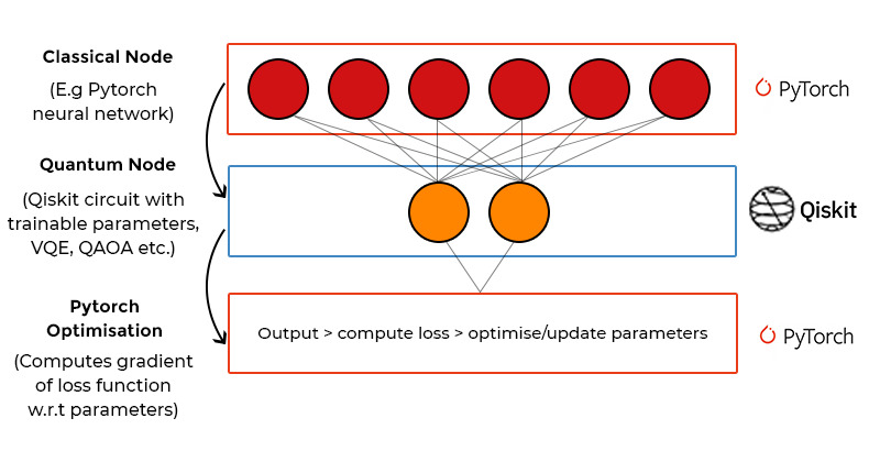
The above image illustrates the framework we’ll build using the following code. Our mission is to create a hybrid quantum-classical neural network that will classify hand-drawn digits. Remember that the edges shown downwards in the image are not indicated in visuals. The directions have been provided for assistance.
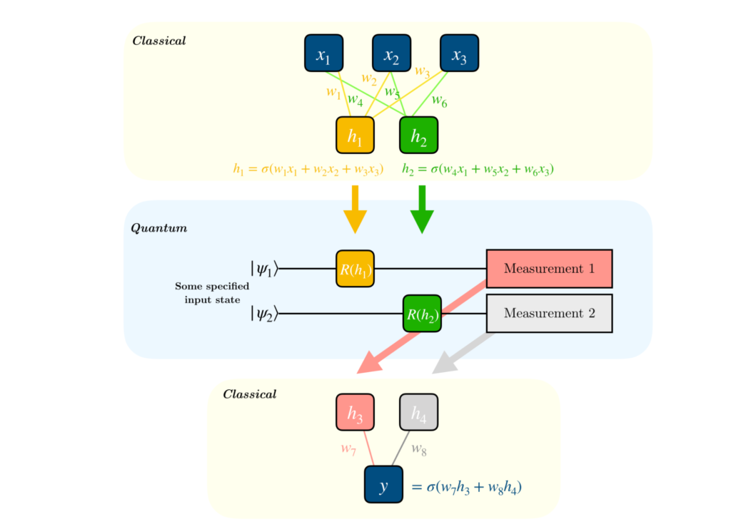
To build a neural network, you need to implement a hidden layer using a parameterized quantum circuit. A parameterized quantum circuit is where the rotation angles are specified by the components of a classical input vector for each gate. The output from the previous layer will be used as an input in the parameterized quantum circuit. The stats are collected from this layer and used as inputs in the next layer. The below diagram explains it clearly.
Those familiar with classical machine learning will want to know how the gradients are calculated in quantum circuits. The step is necessary to assign optimization techniques like gradient descent. While the process is rather technical, we can simplify it a little and explain it as follows:

We can systematically differentiate the quantum circuit in the bigger backpropagation routine. It is known as the parameter shift rule.
Next, we’ll see how to implement a quantum hybrid neural network in Python using the Google Colab environment.
Step1: Install necessary libraries in python
Pip install qiskit
Pip install pytorch
#Note: If you have already working in colab notebook there is no need
Step2: Import necessary libraries in Colab or python framework
import numpy as np
import matplotlib.pyplot as plt
import torch
from torch.autograd import Function
from torchvision import datasets, transforms
import torch.optim as optim
import torch.nn as nn
import torch.nn.functional as F
import qiskit
from qiskit import transpile, assemble
from qiskit.visualization import *
Step3: Create a “Quantum Class” with Qiskit
class QuantumCircuit:
"""
This class provides a simple interface for interaction
with the quantum circuit
"""
def __init__(self, n_qubits, backend, shots):
# --- Circuit definition ---
self._circuit = qiskit.QuantumCircuit(n_qubits)
all_qubits = [i for i in range(n_qubits)]
self.theta = qiskit.circuit.Parameter('theta')
self._circuit.h(all_qubits)
self._circuit.barrier()
self._circuit.ry(self.theta, all_qubits)
self._circuit.measure_all()
# ---------------------------
self.backend = backend
self.shots = shots
def run(self, thetas):
t_qc = transpile(self._circuit,
self.backend)
qobj = assemble(t_qc,
shots=self.shots,
parameter_binds = [{self.theta: theta} for theta in thetas])
job = self.backend.run(qobj)
result = job.result().get_counts()
counts = np.array(list(result.values()))
states = np.array(list(result.keys())).astype(float)
# Compute probabilities for each state
probabilities = counts / self.shots
# Get state expectation
expectation = np.sum(states * probabilities)
return np.array([expectation])
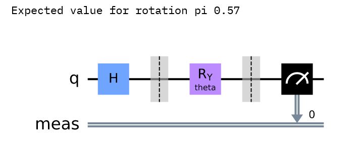
Let’s test the implementation
simulator = qiskit.Aer.get_backend('aer_simulator')
circuit = QuantumCircuit(1, simulator, 100)
print('Expected value for rotation pi {}'.format(circuit.run([np.pi])[0]))
circuit._circuit.draw()
Output:
Step4: Create a “Quantum-Classical Class” with PyTorch
class HybridFunction(Function):
""" Hybrid quantum - classical function definition """
@staticmethod
def forward(ctx, input, quantum_circuit, shift):
""" Forward pass computation """
ctx.shift = shift
ctx.quantum_circuit = quantum_circuit
expectation_z = ctx.quantum_circuit.run(input[0].tolist())
result = torch.tensor([expectation_z])
ctx.save_for_backward(input, result)
return result
@staticmethod
def backward(ctx, grad_output):
""" Backward pass computation """
input, expectation_z = ctx.saved_tensors
input_list = np.array(input.tolist())
shift_right = input_list + np.ones(input_list.shape) * ctx.shift
shift_left = input_list - np.ones(input_list.shape) * ctx.shift
gradients = []
for i in range(len(input_list)):
expectation_right = ctx.quantum_circuit.run(shift_right[i])
expectation_left = ctx.quantum_circuit.run(shift_left[i])
gradient = torch.tensor([expectation_right]) - torch.tensor([expectation_left])
gradients.append(gradient)
gradients = np.array([gradients]).T
return torch.tensor([gradients]).float() * grad_output.float(), None, None
class Hybrid(nn.Module):
""" Hybrid quantum - classical layer definition """
def __init__(self, backend, shots, shift):
super(Hybrid, self).__init__()
self.quantum_circuit = QuantumCircuit(1, backend, shots)
self.shift = shift
def forward(self, input):
return HybridFunction.apply(input, self.quantum_circuit, self.shift)
Step5: Data Loading and Preprocessing
Our idea is to create a simple hybrid neural network that classifies images of the digits 0 and 1 from the MNIST dataset. The foremost thing to do is to load MNIST and filter all the pictures with 0’s and 1’s. We’ll use these as inputs in our neural network.
Training Data codes:
# Concentrating on the first 100 samples
n_samples = 100
X_train = datasets.MNIST(root='./data', train=True, download=True,
transform=transforms.Compose([transforms.ToTensor()]))
# Leaving only labels 0 and 1
idx = np.append(np.where(X_train.targets == 0)[0][:n_samples],
np.where(X_train.targets == 1)[0][:n_samples])
X_train.data = X_train.data[idx]
X_train.targets = X_train.targets[idx]
train_loader = torch.utils.data.DataLoader(X_train, batch_size=1, shuffle=True)
n_samples_show = 6
data_iter = iter(train_loader)
fig, axes = plt.subplots(nrows=1, ncols=n_samples_show, figsize=(10, 3))
while n_samples_show > 0:
images, targets = data_iter.__next__()
axes[n_samples_show - 1].imshow(images[0].numpy().squeeze(), cmap='gray')
axes[n_samples_show - 1].set_xticks([])
axes[n_samples_show - 1].set_yticks([])
axes[n_samples_show - 1].set_title("Labeled: {}".format(targets.item()))
n_samples_show -= 1
Testing Data codes:
n_samples = 50
X_test = datasets.MNIST(root='./data', train=False, download=True,
transform=transforms.Compose([transforms.ToTensor()]))
idx = np.append(np.where(X_test.targets == 0)[0][:n_samples],
np.where(X_test.targets == 1)[0][:n_samples])
X_test.data = X_test.data[idx]
X_test.targets = X_test.targets[idx]
test_loader = torch.utils.data.DataLoader(X_test, batch_size=1, shuffle=True)
Step6: Creating the Hybrid Neural Network
class Net(nn.Module):
def __init__(self):
super(Net, self).__init__()
self.conv1 = nn.Conv2d(1, 6, kernel_size=5)
self.conv2 = nn.Conv2d(6, 16, kernel_size=5)
self.dropout = nn.Dropout2d()
self.fc1 = nn.Linear(256, 64)
self.fc2 = nn.Linear(64, 1)
self.hybrid = Hybrid(qiskit.Aer.get_backend('aer_simulator'), 100, np.pi / 2)
def forward(self, x):
x = F.relu(self.conv1(x))
x = F.max_pool2d(x, 2)
x = F.relu(self.conv2(x))
x = F.max_pool2d(x, 2)
x = self.dropout(x)
x = x.view(1, -1)
x = F.relu(self.fc1(x))
x = self.fc2(x)
x = self.hybrid(x)
return torch.cat((x, 1 - x), -1)
Step7: Training the Network
model = Net()
optimizer = optim.Adam(model.parameters(), lr=0.001)
loss_func = nn.NLLLoss()
epochs = 20
loss_list = []
model.train()
for epoch in range(epochs):
total_loss = []
for batch_idx, (data, target) in enumerate(train_loader):
optimizer.zero_grad()
# Forward pass
output = model(data)
# Calculating loss
loss = loss_func(output, target)
# Backward pass
loss.backward()
# Optimize the weights
optimizer.step()
total_loss.append(loss.item())
loss_list.append(sum(total_loss)/len(total_loss))
print('Training [{:.0f}%]\tLoss: {:.4f}'.format(
100. * (epoch + 1) / epochs, loss_list[-1]))
Output:
Training [5%] Loss: -0.7741
Training [10%] Loss: -0.9155
Training [15%] Loss: -0.9489
Training [20%] Loss: -0.9400
Training [25%] Loss: -0.9496
Training [30%] Loss: -0.9561
Training [35%] Loss: -0.9627
Training [40%] Loss: -0.9499
Training [45%] Loss: -0.9664
Training [50%] Loss: -0.9676
Training [55%] Loss: -0.9761
Training [60%] Loss: -0.9790
Training [65%] Loss: -0.9846
Training [70%] Loss: -0.9836
Training [75%] Loss: -0.9857
Training [80%] Loss: -0.9877
Training [85%] Loss: -0.9895
Training [90%] Loss: -0.9912
Training [95%] Loss: -0.9936
Training [100%] Loss: -0.9901
Plot the training graph
plt.plot(loss_list)
plt.title('Hybrid NN Training Convergence')
plt.xlabel('Training Iterations')
plt.ylabel('Neg Log Likelihood Loss')
Step8: Testing the Network
model.eval()
with torch.no_grad():
correct = 0
for batch_idx, (data, target) in enumerate(test_loader):
output = model(data)
pred = output.argmax(dim=1, keepdim=True)
correct += pred.eq(target.view_as(pred)).sum().item()
loss = loss_func(output, target)
total_loss.append(loss.item())
print('Performance on test data:\n\tLoss: {:.4f}\n\tAccuracy: {:.1f}%'.format(
sum(total_loss) / len(total_loss),
correct / len(test_loader) * 100)
)
Output:
Performance on test data:
Loss: -0.9827
Accuracy: 100.0%
Testing Output:
n_samples_show = 6
count = 0
fig, axes = plt.subplots(nrows=1, ncols=n_samples_show, figsize=(10, 3))
model.eval()
with torch.no_grad():
for batch_idx, (data, target) in enumerate(test_loader):
if count == n_samples_show:
break
output = model(data)
pred = output.argmax(dim=1, keepdim=True)
axes[count].imshow(data[0].numpy().squeeze(), cmap='gray')
axes[count].set_xticks([])
axes[count].set_yticks([])
axes[count].set_title('Predicted {}'.format(pred.item()))
        count += 1

Code source: Github
Considering the research going on in the field of quantum computing and its applications in artificial intelligence, we can expect faster progress and better results in the near future. We’ll see many more quantum computers on the cloud as it is a feasible and cost-effective solution for everyone in the industry.
Though quantum computers might not replace classical computers, businesses will use quantum computers along with classical computers to optimize the processes and achieve their goals.
