In today’s world of deep learning, transfer learning is a well-versed technique to train artificial neural networks. One of the major reasons is that it is good at solving complex problems and another is the need for less training data.
The recent developments in Quantum computing opens some new areas such as Quantum machine learning which leverages the power of quantum computing with traditional neural network to enhance its accuracy and help in exploring new patterns in the data.
In this article, we will deeply explore the power of Quantum transfer learning and where it can be utilized. We will also show how to implement a variational quantum circuit to use quantum principles with transfer learning. Before going into depth, we need to get an understanding of what is transfer learning and its related terminologies
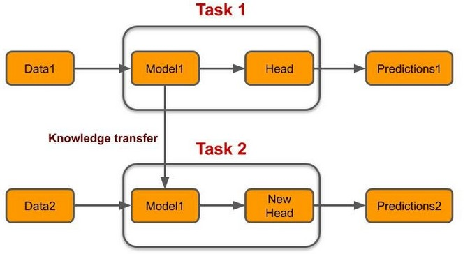
In quantum transfer learning, the core concept involves transferring knowledge or insights acquired from one quantum task to another, even if the tasks are distinct. This knowledge transfer serves to enhance the performance or expedite the learning process for the target quantum task. A significant departure from classical transfer learning lies in the replacement of LSTM cells with variational quantum circuits, a unique type of quantum circuit.
For better understanding, we should be familiar with the basics of neural networks, transfer learning, and some basics of Quantum computing.
Transfer learning (TL) is a technique in machine learning (ML) in which knowledge learned from a task is re-used to boost performance on a related task. For example, for image classification, knowledge gained while learning to recognize cars could be applied when trying to recognize trucks. This topic is associated with the psychological literature on transfer of learning, although practical ties between the two fields are limited. Reusing/transferring information from previously learned tasks to new tasks has the potential to improve learning efficiency significantly.
The term ‘Quantum’ comes from Quantum Mechanics, which is the study of the physical properties of the nature of electrons and photons in physics. It is a framework to describe and understand the complexities of nature. Quantum computing is the process of using quantum mechanics to solve highly complicated problems.
We use classic computing to solve problems that are difficult for humans to solve. Now, we use quantum computing to solve problems that classic computing cannot solve. Quantum computing works on a huge volume of complex data in quick time.
Superposition is when the quantum system is present in more than one state at the same time. It’s an inherent ability of the quantum system. We can consider the time machine as an example to explain superposition. The person in the time machine is present in more than one place at the same time. Similarly, when a particle is present in multiple states at once, it is called superposition.
Entanglement is the correlation between the quantum particles. The particles are connected in a way that even if they were present at the opposite ends of the world, they’ll still be in sync and ‘dance’ simultaneously. The distance between the particles doesn’t matter as the entanglement between them is very strong. Einstein had described this phenomenon as ‘spooky action at a distance.
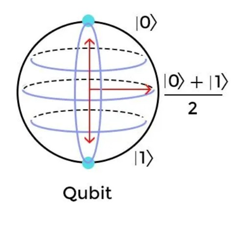
A quantum bit is a measure of data storage unit in quantum computers. The quantum bit is a subatomic particle that can be made of electrons or photons. Every quantum bit or Qbit adheres to the principles of superposition and entanglement. This makes things hard for scientists to generate Qbits and manage them. That’s because Qbits can show multiple combinations of zeros and ones (0 & 1) at the same time (superposition).
Quantum transfer learning is a concept that draws inspiration from classical machine learning and transfer learning but is applied in the context of quantum computing. Quantum computing leverages the principles of quantum mechanics to perform certain computational tasks more efficiently than classical computers.
In the context of quantum transfer learning, the idea is to transfer knowledge or information learned from one quantum task to another, potentially different quantum task. This transfer of knowledge can help in improving the performance or speeding up the learning process for the target quantum task.
One of the major differences between classical transfer learning and Quantum transfer learning is here we are replacing LSTM cells with variational quantum circuits which are a kind of quantum circuit.
Here is a basic workflow of Quantum transfer learning:
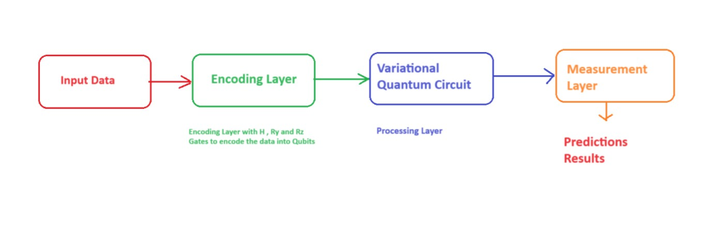
The architecture of Quantum transfer learning is given below:

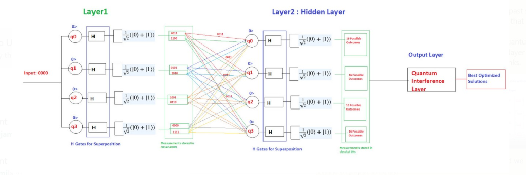
Quantum transfer learning has the potential to address challenges in quantum machine learning, such as the limited availability of quantum training data and the computational cost of training quantum models from scratch. By transferring knowledge from related tasks, it may be possible to achieve better results and accelerate the development of quantum algorithms.
It’s important to note that quantum transfer learning is an emerging field, and its practical applications and effectiveness are still being explored. As quantum computing technology advances, we can expect more research and developments in this area.
Quantum transfer learning, although an emerging concept, holds promise for a variety of use cases in quantum computing and machine learning. Some potential use cases include:
Transfer learning can be applied to quantum chemistry problems. For instance, knowledge gained from simulating the electronic structure of one molecule can be transferred to another molecule, accelerating the calculation of quantum properties.
Quantum transfer learning can be used to enhance quantum optimization tasks. Knowledge from solving one optimization problem can be transferred to solve similar problems more efficiently.
In quantum image processing, knowledge learned from one type of image analysis task can be transferred to others, such as object recognition, image denoising, or image segmentation.
Transfer learning can be valuable in QNLP tasks. Information gained from one quantum NLP task (e.g., sentiment analysis) can be transferred to another (e.g., language translation), improving efficiency and performance.
Quantum transfer learning can be applied to robotics and control tasks. Knowledge learned from controlling one type of quantum system can be transferred to control other quantum systems.
In quantum generative modeling, such as quantum variational autoencoders (Q-VAEs), transfer learning can help generate new quantum states or molecules based on knowledge from previously learned states.
In quantum computing, transfer learning can be used to improve the compilation of quantum circuits. Techniques learned from compiling one set of quantum algorithms can be applied to compile other quantum algorithms more efficiently.
Knowledge from compressing one quantum dataset can be transferred to compress other datasets, reducing the quantum resources required for storage and transmission.
In quantum anomaly detection tasks, transfer learning can be employed to identify anomalies in quantum systems based on patterns learned from other related quantum systems.
In quantum finance, knowledge gained from predicting financial market trends for one asset or market can be transferred to make predictions for other assets or markets.
In this, we will use classical to quantum transfer learning on an image dataset and then we will do some image classifications.
import time
import os
import copy
# PyTorch
import torch
import torch.nn as nn
import torch.optim as optim
from torch.optim import lr_scheduler
import torchvision
from torchvision import datasets, transforms
# Pennylane
import pennylane as qml
from pennylane import numpy as np
torch.manual_seed(42)
np.random.seed(42)
# Plotting
import matplotlib.pyplot as plt
# OpenMP: number of parallel threads.
os.environ["OMP_NUM_THREADS"] = "1"
n_qubits = 4 # Number of qubits
step = 0.0004 # Learning rate
batch_size = 4 # Number of samples for each training step
num_epochs = 3 # Number of training epochs
q_depth = 6 # Depth of the quantum circuit (number of variational layers)
gamma_lr_scheduler = 0.1 # Learning rate reduction applied every 10 epochs.
q_delta = 0.01 # Initial spread of random quantum weights
start_time = time.time() # Start of the computation timer
dev = qml.device("default.qubit", wires=n_qubits)
device = torch.device("cuda:0" if torch.cuda.is_available() else "cpu")
data_transforms = {
"train": transforms.Compose(
[
# transforms.RandomResizedCrop(224), # uncomment for data augmentation
# transforms.RandomHorizontalFlip(), # uncomment for data augmentation
transforms.Resize(256),
transforms.CenterCrop(224),
transforms.ToTensor(),
# Normalize input channels using mean values and standard deviations of ImageNet.
transforms.Normalize([0.485, 0.456, 0.406], [0.229, 0.224, 0.225]),
]
),
"val": transforms.Compose(
[
transforms.Resize(256),
transforms.CenterCrop(224),
transforms.ToTensor(),
transforms.Normalize([0.485, 0.456, 0.406], [0.229, 0.224, 0.225]),
]
),
}
data_dir = "../_data/hymenoptera_data"
image_datasets = {
x if x == "train" else "validation": datasets.ImageFolder(
os.path.join(data_dir, x), data_transforms[x]
)
for x in ["train", "val"]
}
dataset_sizes = {x: len(image_datasets[x]) for x in ["train", "validation"]}
class_names = image_datasets["train"].classes
# Initialize dataloader
dataloaders = {
x: torch.utils.data.DataLoader(image_datasets[x], batch_size=batch_size, shuffle=True)
for x in ["train", "validation"]
}
# function to plot images
def imshow(inp, title=None):
"""Display image from tensor."""
inp = inp.numpy().transpose((1, 2, 0))
# Inverse of the initial normalization operation.
mean = np.array([0.485, 0.456, 0.406])
std = np.array([0.229, 0.224, 0.225])
inp = std * inp + mean
inp = np.clip(inp, 0, 1)
plt.imshow(inp)
if title is not None:
plt.title(title)
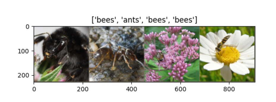
def H_layer(nqubits):
"""Layer of single-qubit Hadamard gates.
"""
for idx in range(nqubits):
qml.Hadamard(wires=idx)
def RY_layer(w):
"""Layer of parametrized qubit rotations around the y axis.
"""
for idx, element in enumerate(w):
qml.RY(element, wires=idx)
def entangling_layer(nqubits):
"""Layer of CNOTs followed by another shifted layer of CNOT.
"""
# In other words it should apply something like :
# CNOT CNOT CNOT CNOT... CNOT
# CNOT CNOT CNOT... CNOT
for i in range(0, nqubits - 1, 2): # Loop over even indices: i=0,2,...N-2
qml.CNOT(wires=[i, i + 1])
for i in range(1, nqubits - 1, 2): # Loop over odd indices: i=1,3,...N-3
qml.CNOT(wires=[i, i + 1])
@qml.qnode(dev, interface="torch")
def quantum_net(q_input_features, q_weights_flat):
"""
The variational quantum circuit.
"""
# Reshape weights
q_weights = q_weights_flat.reshape(q_depth, n_qubits)
# Start from state |+> , unbiased w.r.t. |0> and |1>
H_layer(n_qubits)
# Embed features in the quantum node
RY_layer(q_input_features)
# Sequence of trainable variational layers
for k in range(q_depth):
entangling_layer(n_qubits)
RY_layer(q_weights[k])
# Expectation values in the Z basis
exp_vals = [qml.expval(qml.PauliZ(position)) for position in range(n_qubits)]
return tuple(exp_vals)
class DressedQuantumNet(nn.Module):
"""
Torch module implementing the *dressed* quantum net.
"""
def __init__(self):
"""
Definition of the *dressed* layout.
"""
super().__init__()
self.pre_net = nn.Linear(512, n_qubits)
self.q_params = nn.Parameter(q_delta * torch.randn(q_depth * n_qubits))
self.post_net = nn.Linear(n_qubits, 2)
def forward(self, input_features):
"""
Defining how tensors are supposed to move through the *dressed* quantum
net.
"""
# obtain the input features for the quantum circuit
# by reducing the feature dimension from 512 to 4
pre_out = self.pre_net(input_features)
q_in = torch.tanh(pre_out) * np.pi / 2.0
# Apply the quantum circuit to each element of the batch and append to q_out
q_out = torch.Tensor(0, n_qubits)
q_out = q_out.to(device)
for elem in q_in:
q_out_elem = torch.hstack(quantum_net(elem, self.q_params)).float().unsqueeze(0)
q_out = torch.cat((q_out, q_out_elem))
# return the two-dimensional prediction from the postprocessing layer
return self.post_net(q_out)
model_hybrid = torchvision.models.resnet18(pretrained=True)
for param in model_hybrid.parameters():
param.requires_grad = False
# Notice that model_hybrid.fc is the last layer of ResNet18
model_hybrid.fc = DressedQuantumNet()
# Use CUDA or CPU according to the "device" object.
model_hybrid = model_hybrid.to(device)

criterion = nn.CrossEntropyLoss()
optimizer_hybrid = optim.Adam(model_hybrid.fc.parameters(), lr=step)
exp_lr_scheduler = lr_scheduler.StepLR(
optimizer_hybrid, step_size=10, gamma=gamma_lr_scheduler
)
def train_model(model, criterion, optimizer, scheduler, num_epochs):
since = time.time()
best_model_wts = copy.deepcopy(model.state_dict())
best_acc = 0.0
best_loss = 10000.0 # Large arbitrary number
best_acc_train = 0.0
best_loss_train = 10000.0 # Large arbitrary number
print("Training started:")
for epoch in range(num_epochs):
# Each epoch has a training and validation phase
for phase in ["train", "validation"]:
if phase == "train":
# Set model to training mode
model.train()
else:
# Set model to evaluate mode
model.eval()
running_loss = 0.0
running_corrects = 0
# Iterate over data.
n_batches = dataset_sizes[phase] // batch_size
it = 0
for inputs, labels in dataloaders[phase]:
since_batch = time.time()
batch_size_ = len(inputs)
inputs = inputs.to(device)
labels = labels.to(device)
optimizer.zero_grad()
# Track/compute gradient and make an optimization step only when training
with torch.set_grad_enabled(phase == "train"):
outputs = model(inputs)
_, preds = torch.max(outputs, 1)
loss = criterion(outputs, labels)
if phase == "train":
loss.backward()
optimizer.step()
# Print iteration results
running_loss += loss.item() * batch_size_
batch_corrects = torch.sum(preds == labels.data).item()
running_corrects += batch_corrects
print(
"Phase: {} Epoch: {}/{} Iter: {}/{} Batch time: {:.4f}".format(
phase,
epoch + 1,
num_epochs,
it + 1,
n_batches + 1,
time.time() - since_batch,
),
end="\r",
flush=True,
)
it += 1
# Print epoch results
epoch_loss = running_loss / dataset_sizes[phase]
epoch_acc = running_corrects / dataset_sizes[phase]
print(
"Phase: {} Epoch: {}/{} Loss: {:.4f} Acc: {:.4f} ".format(
"train" if phase == "train" else "validation ",
epoch + 1,
num_epochs,
epoch_loss,
epoch_acc,
)
)
# Check if this is the best model wrt previous epochs
if phase == "validation" and epoch_acc > best_acc:
best_acc = epoch_acc
best_model_wts = copy.deepcopy(model.state_dict())
if phase == "validation" and epoch_loss < best_loss:
best_loss = epoch_loss
if phase == "train" and epoch_acc > best_acc_train:
best_acc_train = epoch_acc
if phase == "train" and epoch_loss < best_loss_train:
best_loss_train = epoch_loss
# Update learning rate
if phase == "train":
scheduler.step()
# Print final results
model.load_state_dict(best_model_wts)
time_elapsed = time.time() - since
print(
"Training completed in {:.0f}m {:.0f}s".format(time_elapsed // 60, time_elapsed % 60)
)
print("Best test loss: {:.4f} | Best test accuracy: {:.4f}".format(best_loss, best_acc))
return model
model_hybrid = train_model(
model_hybrid, criterion, optimizer_hybrid, exp_lr_scheduler, num_epochs=num_epochs
)
def visualize_model(model, num_images=6, fig_name="Predictions"):
images_so_far = 0
_fig = plt.figure(fig_name)
model.eval()
with torch.no_grad():
for _i, (inputs, labels) in enumerate(dataloaders["validation"]):
inputs = inputs.to(device)
labels = labels.to(device)
outputs = model(inputs)
_, preds = torch.max(outputs, 1)
for j in range(inputs.size()[0]):
images_so_far += 1
ax = plt.subplot(num_images // 2, 2, images_so_far)
ax.axis("off")
ax.set_title("[{}]".format(class_names[preds[j]]))
imshow(inputs.cpu().data[j])
if images_so_far == num_images:
return
visualize_model(model_hybrid, num_images=batch_size)
plt.show()
To recap, we got into a concise exploration of the following key points:
It’s important to note that quantum transfer learning is still an evolving field, and its practical applicability depends on the development of quantum hardware and algorithms. As quantum computing technology advances, we can expect to see more diverse and sophisticated applications of quantum transfer learning across various domains.
